Planet Money Panel on Financial Innovation

Tyler Cowen, Felix Salmon, and Rortybomb duke it out on Planet Money:
http://www.npr.org/blogs/money/2009/08/podcast_where_financial_innova.html

Sqlite and SqlAlchemy

Although I’m beginning to think that it may make more sense to use something like PyTables to store time series data, it’s hard to escape the ubiquity of relational databases in the enterprise. In tightly controlled corporate environments, PyTables might not even be an option. Since I’m on a database kick, I thought I might as well investigate ORMs (object relational mappers) and see whether they make sense (from an analyst perspective). SQLAlchemy (SQLA) is one of the big kahunas in the python community, though there are clearly many others (Django ORM, SqlObject, etc.).

I’ve come to realize SQLAlchemy doesn’t promise that you’ll write less code. It just promises that the additional code you write (when necessary) will be worth the additional power and flexibility it provides. SQLAlchemy allows the user to leverage the powerful idioms of the python language, provides a consistent “API” for multiple databases, and automates many database housekeeping details (e.g. transactions, joins, etc.). It also offers powerful reflection features that make accessing legacy databases simple. Furthermore, SQLAlchemy features an SQL expression language separate from the ORM so users can choose between SQL-like syntax or objects when appropriate, allowing the user to map tables to classes at will. Other ORMs bind tables and classes together tightly (a la the ActiveRecord pattern featured in Rails and other ORMs).

The documentation for SqlAlchemy is mostly good. It’s good because it exists, it’s maintained, and documents the complete API. The tutorials are instructive, but I felt they were a bit hard to follow since the author attempts to highlight different ways to do the same thing. This conflation of demo and tutorial makes it harder to keep track of what exactly needs to be instantiated and when. A separate interactive demo screencast + a more linear tutorial might have worked better.

Anyway, I won’t cover SqlAlchemy’s Expression Language here, it’s available in the documentation and should make sense to those already familiar with SQL. The expression language essentially transforms SQL into method calls (e.g. “table.insert().values(values)” rather than “INSERT INTO table (fields) VALUES (values)”).

So, using matplotlib’s handy quote_historical_yahoo() function, we can replicate the database from a previous post using SqlAlchemy’s declarative plugin. The declarative plugin allows the user to map tables to objects in a single step. The following code defines two tables, “assets” and “prices,” and defines a function for pulling data for a given ticker from yahoo (adapted from the previous post on sqlite and python).

'''
SQLAlchemy ORM declarative example.
'''

from sqlalchemy.ext.declarative import declarative_base
from sqlalchemy import Table, Column, Integer, String, DECIMAL
from sqlalchemy import MetaData, create_engine, ForeignKey
from sqlalchemy.orm import relation, backref, sessionmaker, scoped_session
from matplotlib.finance import quotes_historical_yahoo
import datetime
import os

path = os.path.expanduser('~')  + \
 '/Dev/Data/AssetPrices/SQLite/assetprices_SA.sqlite'
engine = create_engine('sqlite:////' + path, echo=True)
Base = declarative_base(bind=engine)

date1 = datetime.datetime(2009,1,1)
date2 = datetime.datetime.now()

#DEFINE TABLES#

class Asset(Base):
 __tablename__ = 'assets'

 asset_id = Column(Integer, primary_key=True)
 ticker = Column(String, unique=True)
 tag = Column(String)

 prices = relation('Price', order_by='Price.gregorian_day', backref='assets')

 def __init__(self, ticker, tag):
 self.ticker = ticker
 self.tag = tag

 def __repr__(self):
 return "<Asset('%s', '%s')>" % (self.ticker, self.tag)

class Price(Base):
 __tablename__ = 'prices'

 price_id = Column(Integer, primary_key=True)
 asset_id = Column(Integer, ForeignKey('assets.asset_id'))
 gregorian_day = Column(Integer)
 date_string = Column(String)
 year = Column(Integer)
 month = Column(Integer)
 day = Column(Integer)
 px_open = Column(DECIMAL)
 px_close = Column(DECIMAL)
 px_high = Column(DECIMAL)
 px_low = Column(DECIMAL)
 volume = Column(Integer)

 #asset = relation(Asset, backref=backref('prices',
 #order_by=gregorian_day))

 def __init__(self, gregorian_day, date_string, year, month, day,
 px_open, px_close, px_high, px_low, volume):
 self.gregorian_day = gregorian_day
 self.date_string = date_string
 self.year = year
 self.month = month
 self.day = day
 self.px_open = px_open
 self.px_close = px_close
 self.px_high = px_high
 self.px_low = px_low
 self.volume = volume

 def __repr__(self):
 return "<Price('%s', '%s', '%s','%s','%s','%s','%s','%s','%s','%s')>" \
 % (self.gregorian_day, self.date_string, self.year, self.month,
 self.day, self.px_open, self.px_close, self.px_high,
 self.px_low, self.volume)

#CREATE DB TABLES#

Base.metadata.create_all(engine)

#PACKAGE RAW DATA#

def package_data(db=None, ticker=None, tag='stock', start=None, end=None):
 '''
 package_data() uses quotes_historical_yahoo() to create a data set for a
 given stock's price history. Date_string, Year, month, and day fields are
 included for added flexibility. Returns a dictionary of tuples.
 '''
 raw_quotes = quotes_historical_yahoo(ticker, start, end) #list of tuples

 data = []
 for quote in raw_quotes:
 date_raw = datetime.datetime.fromordinal(int(quote[0]))
 year, month, day = date_raw.year, date_raw.month, date_raw.day
 date_string = date_raw.strftime("%Y-%m-%d")
 record = (ticker, tag, quote[0], date_string, year, month, day,
 quote[1], quote[2], quote[3], quote[4], quote[5])
 data.append(record)    

 headers = ('ticker',
 'tag',
 'gregorian_day',
 'date_string',
 'year',
 'month',
 'day',
 'px_open',
 'px_close',
 'px_high',
 'px_low',
 'volume')
 return {'data':data, 'headers':headers}

Executing this code essentially sets up the schema for an sqlite database and provides a package_data() function that will pull in data for a given ticker and date range. The “echo=True” parameter in  “engine = create_engine(‘sqlite:////’ + path, echo=True)” will print out the SQL statements SQLA generates to the terminal.

Executing the code yields:

>>>
Evaluating SAscratchcode.py
2009-08-14 00:58:57,862 INFO sqlalchemy.engine.base.Engine.0x…b9b0 PRAGMA table_info(“assets”)
2009-08-14 00:58:57,863 INFO sqlalchemy.engine.base.Engine.0x…b9b0 ()
2009-08-14 00:58:57,863 INFO sqlalchemy.engine.base.Engine.0x…b9b0 PRAGMA table_info(“prices”)
2009-08-14 00:58:57,863 INFO sqlalchemy.engine.base.Engine.0x…b9b0 ()
2009-08-14 00:58:57,864 INFO sqlalchemy.engine.base.Engine.0x…b9b0
CREATE TABLE assets (
asset_id INTEGER NOT NULL,
ticker VARCHAR,
tag VARCHAR,
PRIMARY KEY (asset_id),
UNIQUE (ticker)
)2009-08-14 00:58:57,864 INFO sqlalchemy.engine.base.Engine.0x…b9b0 ()
2009-08-14 00:58:57,865 INFO sqlalchemy.engine.base.Engine.0x…b9b0 COMMIT
2009-08-14 00:58:57,866 INFO sqlalchemy.engine.base.Engine.0x…b9b0
CREATE TABLE prices (
price_id INTEGER NOT NULL,
asset_id INTEGER,
gregorian_day INTEGER,
date_string VARCHAR,
year INTEGER,
month INTEGER,
day INTEGER,
px_open NUMERIC(10, 2),
px_close NUMERIC(10, 2),
px_high NUMERIC(10, 2),
px_low NUMERIC(10, 2),
volume INTEGER,
PRIMARY KEY (price_id),
FOREIGN KEY(asset_id) REFERENCES assets (asset_id)
)

2009-08-14 00:58:57,866 INFO sqlalchemy.engine.base.Engine.0x…b9b0 ()
2009-08-14 00:58:57,868 INFO sqlalchemy.engine.base.Engine.0x…b9b0 COMMIT

This output shouldn’t be too surprising. We’ve basically just created the tables we defined. So let’s experiment interactively and create an asset object for Google.

>>> GOOG=Asset(‘GOOG’, ‘stock’)
>>> GOOG
<Asset(‘GOOG’, ‘stock’)>
>>> GOOG.ticker
‘GOOG’

As you can see, it’s possible now to call attributes of the GOOG object by name (e.g. ticker).

In our table definitions, we used SQLA’s relation() function (e.g. prices = relation(‘Price’, order_by=’Price.gregorian_day’, backref=’assets’)) to define a one-to-many relationship between an asset and its prices. SQLA uses the foreign key defined in the prices table to automatically generate the correct SQL. This is particularly interesting for sqlite users as sqlite parses foreign key statements but does not enforce them. Using this relation function, we can actually use dot notation to look at the GOOG object’s prices attribute, just as if the prices are part of the object.

>>> GOOG.prices
[]

The prices are represented by an empty list since we haven’t actually written any prices into the database yet. So insert some prices.

>>> raw = package_data(ticker=’GOOG’, start=date1, end=date2)
>>> raw[‘headers’]
(‘ticker’, ‘tag’, ‘gregorian_day’, ‘date_string’, ‘year’, ‘month’, ‘day’, ‘px_open’, ‘px_close’, ‘px_high’, ‘px_low’, ‘volume’)

The package_data() function returns a python dictionary, {‘data’:[(list of tuples)], ‘headers’,(tuple of headers)}. So how do we assign the prices to the right ticker? The obvious way to do it would be to use a list comprehension to create a list of Price objects, and assign them to the GOOG object’s “prices” attribute.

>>> GOOG.prices = [Price(record[2],record[3],record[4], record[5],record[6],record[7],record[8],record[9],record[10],record[11]) for record in raw[‘data’]]
>>> GOOG.prices
[<Price(‘733409.0’, ‘2009-01-02’, ‘2009’,’1′,’2′,’308.6′,’321.32′,’321.82′,’305.5′,’3610500′)>,
<Price(‘733412.0’, ‘2009-01-05’, ‘2009’,’1′,’5′,’321.0′,’328.05′,’331.24′,’315.0′,’4889000′)>,…]

I’ve just listed the first two records to save some space, but you get the picture. The important thing to recognize here is that no SQL has been issued to the database yet. In order to reduce the back and forth between the database, SQLA uses a Session() object to keep track of what’s going on. So let’s setup a session and add our GOOG object to the session so SQLA can track it.

>>> Session = scoped_session(sessionmaker(engine))
>>> session = Session()
>>> session.add(GOOG)
>>> session.commit()
2009-08-14 01:10:15,424 INFO sqlalchemy.engine.base.Engine.0x…b9b0 BEGIN
2009-08-14 01:10:15,425 INFO sqlalchemy.engine.base.Engine.0x…b9b0 INSERT INTO assets (ticker, tag) VALUES (?, ?)
2009-08-14 01:10:15,425 INFO sqlalchemy.engine.base.Engine.0x…b9b0 [‘GOOG’, ‘stock’]
2009-08-14 01:10:15,471 INFO sqlalchemy.engine.base.Engine.0x…b9b0 INSERT INTO prices (asset_id, gregorian_day, date_string, year, month, day, px_open, px_close, px_high, px_low, volume) VALUES (?, ?, ?, ?, ?, ?, ?, ?, ?, ?, ?)
2009-08-14 01:10:15,471 INFO sqlalchemy.engine.base.Engine.0x…b9b0 [1, 733409.0, ‘2009-01-02’, 2009, 1, 2, ‘308.6’, ‘321.32’, ‘321.82’, ‘305.5’, 3610500]
2009-08-14 01:10:15,472 INFO sqlalchemy.engine.base.Engine.0x…b9b0 INSERT INTO prices (asset_id, gregorian_day, date_string, year, month, day, px_open, px_close, px_high, px_low, volume) VALUES (?, ?, ?, ?, ?, ?, ?, ?, ?, ?, ?)
2009-08-14 01:10:15,472 INFO sqlalchemy.engine.base.Engine.0x…b9b0 [1, 733412.0, ‘2009-01-05’, 2009, 1, 5, ‘321.0’, ‘328.05’, ‘331.24’, ‘315.0’, 4889000]
…(and it continues on)…

So the code above basically creates a session, adds our GOOG object to the session, and then commits all changes. The commit() method signals SQLA to issue all the necessary SQL in a single transaction to our sqlite database. Now that there are actual prices in the database, we can check out GOOG.prices:

>>> GOOG.prices[0]
2009-08-14 01:18:57,881 INFO sqlalchemy.engine.base.Engine.0x…b9b0 BEGIN
2009-08-14 01:18:57,883 INFO sqlalchemy.engine.base.Engine.0x…b9b0 SELECT assets.asset_id AS assets_asset_id, assets.ticker AS assets_ticker, assets.tag AS assets_tag
FROM assets
WHERE assets.asset_id = ?
2009-08-14 01:18:57,883 INFO sqlalchemy.engine.base.Engine.0x…b9b0 [1]
2009-08-14 01:18:57,885 INFO sqlalchemy.engine.base.Engine.0x…b9b0 SELECT prices.price_id AS prices_price_id, prices.asset_id AS prices_asset_id, prices.gregorian_day AS prices_gregorian_day, prices.date_string AS prices_date_string, prices.year AS prices_year, prices.month AS prices_month, prices.day AS prices_day, prices.px_open AS prices_px_open, prices.px_close AS prices_px_close, prices.px_high AS prices_px_high, prices.px_low AS prices_px_low, prices.volume AS prices_volume
FROM prices
WHERE ? = prices.asset_id ORDER BY prices.gregorian_day
2009-08-14 01:18:57,885 INFO sqlalchemy.engine.base.Engine.0x…b9b0 [1]
<Price(‘733409’, ‘2009-01-02’, ‘2009’,’1′,’2′,’308.6′,’321.32′,’321.82′,’305.5′,’3610500′)>

Using normal python slicing syntax, we’ve just called up the first record in the prices table for Google. In this case, SQLA uses “lazy loading” to pull the appropriate Price object by issuing the SQL on demand. Users can choose to ‘eager load’ the data as well. Now that the corresponding Price object has been pulled we can inspect other attributes.

>>> GOOG.prices[0].px_high
Decimal(“321.82”)
>>> test_run = [(record.date_string, record.px_close) for record in GOOG.prices[0:10]]
>>> test_run
[(u’2009-01-02′, Decimal(“321.32”)), (u’2009-01-05′, Decimal(“328.05”)), (u’2009-01-06′, Decimal(“334.06”)), (u’2009-01-07′, Decimal(“322.01”)), (u’2009-01-08′, Decimal(“325.19”)), (u’2009-01-09′, Decimal(“315.07”)), (u’2009-01-12′, Decimal(“312.69”)), (u’2009-01-13′, Decimal(“314.32”)), (u’2009-01-14′, Decimal(“300.97”)), (u’2009-01-15′, Decimal(“298.99”))]

In the example above, we call up the high price for the first record in our table. ‘test_run’ simply creates a list of the first ten date_strings and px_close prices.

Anyway, there’s a lot more to SQLA, this just scratches the surface. We’ll see how deep the rabbit hole goes!

Posted via email from NotesToSelf

Python and Powerpoint

I recently talked to someone who was interested in integrating the different MS-Office products programmatically. The obvious solution is VBA, since it’s built-in. I have no desire to learn VBA, but Python does offer the win32 COM interface. I’d almost forgotten since I’ve been using a Mac for a while. Anyway, I ran across this short tutorial on using COM and Python to automate the creation of powerpoint slides. I used COM with excel a while back, but it was slow (and thus turned to the very nice xlwt/xlrd combo to manipulate excel files). Nevertheless, I can see it coming in handy if you are constantly updating slides with essentially the same, but more recent, data.

Sqlite or Pytables or Text?

I’m wondering whether it makes more sense to store time series data in sqlite or a hierarchical database (like PyTables, which is based on the HDF5 format). Or maybe even straight-up text files!

Sqlite is nice because it runs everywhere and can connect to almost anything. Could serve as the ‘Rosetta Stone‘ for slinging data around.

But PyTables is nice because it integrates with multidimensional numpy arrays and offers object-like convenience, meaning inter-row analysis is probably easier. Pytables is probably faster than sqlite but that’s not really a big concern for me. Both hold plenty of data.

Text files, like CSV, are dead-simple and immediately accessible, but would require more logical work.

Decisions, decisions…

Use python and sqlite3 to build a database

The previous post showed how matplotlib can pull market data from Yahoo. Using some python-fu, you can easily create CSV files for given stocks. CSV files are great as they are easy to parse and don’t require a lot of overhead (in terms of setting things up, you can just open the file directly). Of course, Yahoo, Google, and others offer decent tools to view stock prices, so creating CSV files might be a bit redundant. Furthermore, if you really want to go whole hog and pull prices for thousands of assets, I imagine one would have to think carefully about an appropriate filesystem.

On the other hand, python includes a built in wrapper for sqlite, the ubiquitous file-based database that’s embedded in so many mobile and desktop applications. Sqlite can be run on any platform and is a completely open source, flyweight piece of software (which explains it’s popularity). This post will outline how to create a simple two table sqlite database to store stock prices.

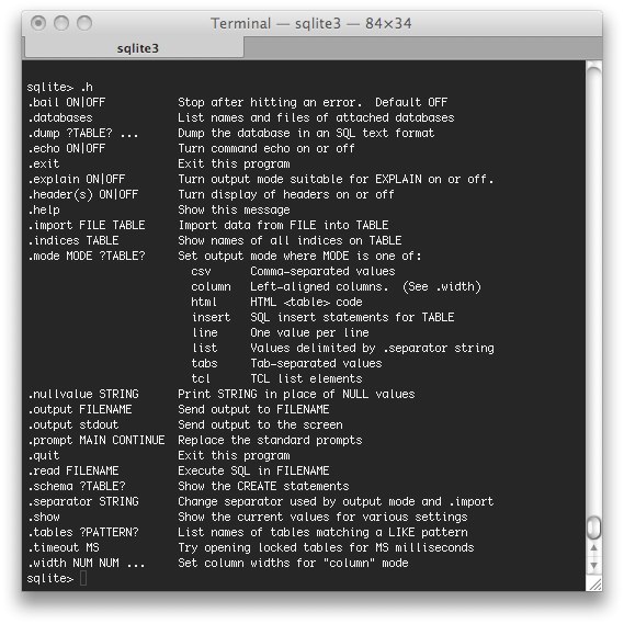
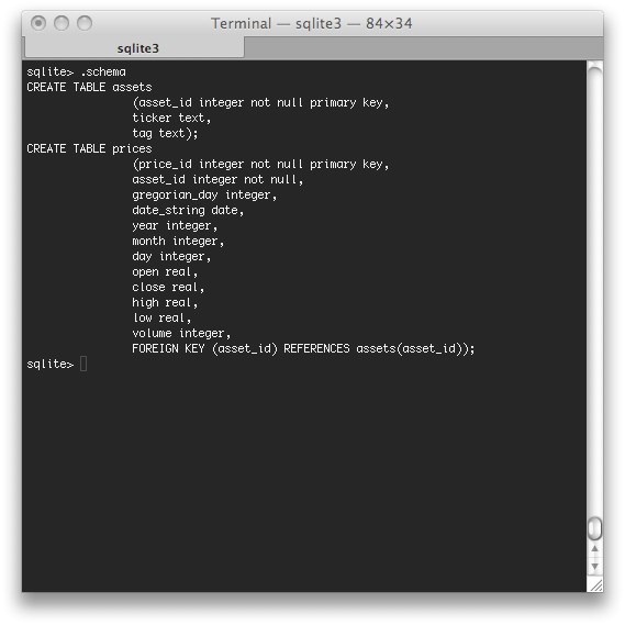
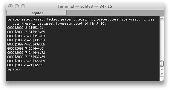
First if all, sqlite has it’s own interpreter you can access from the command line, so if you’re an sql cowboy, you can instantly execute sql statements from the prompt to explore a given database. Here are a few examples:

The .help command lists some of the sqlite specific commands available at the command line.

The .schema command prints the tables in the database (just as you might think).

You can also input sql statements directly.

Anyway, enough about sqlite itself, let’s get to the python that built the database above. The attached script used four functions to package data for a defined set of tickers, using quotes_historical_yahoo(), and inserts the data into an sqlite database. The key is using a dictionary of tuples to pass around data.

stocks = {'data':[('GOOG', 'stock'), ('AAPL','stock')],
 'headers':('ticker', 'tag')}

In the example above, the ‘data’ key references a list of tuples that provide information on the ticker and type of asset in the tuple. The ‘header’ key references the table field names (as defined in the database schema) associated with the ‘data’ key. The same structure is used to write market data to the database, where the ‘data’ key refers to numeric data (e.g., foreign keys, date string, open, close, etc.) and the ‘header’ key refers to the formal fields to which each piece of data is associated.

raw_quotes = quotes_historical_yahoo(ticker, start, end) #list of tuples
data = []
for quote in raw_quotes:
 date_raw = datetime.datetime.fromordinal(int(quote[0]))
 year, month, day = date_raw.year, date_raw.month, date_raw.day
 date_string = str(year)+'-'+str(month)+'-'+str(day)
 record = (f_key, quote[0], date_string, year, month, day,
 quote[1], quote[2], quote[3], quote[4], quote[5])
 data.append(record)    

headers = ('asset_id',
 'gregorian_day',
 'date_string',
 'year',
 'month',
 'day',
 'open',
 'close',
 'high',
 'low',
 'volume')
return {'data':data, 'headers':headers}

I use a fair amount of string substitution in the code, which isn’t strictly recommended, but I’m not particularly worried about security. Anyway, the write2sql() function needs to know how many fields are associated with the data. Rather than create two separate functions for adding stocks to the asset table and market data to the prices table, I used string operations to expand or contract the substitution marks to match the number of headers. I’m sure there are more elegant ways to do it, but, hey, it works.

Finally, I’ll plug the Sqlite Manager add-on for Firefox. It’s a basic and easy way to inspect sqlite files.

Here’s the complete code:

quotes_historical_yahoo from matplotlib.finance

I thought matplotlib was purely a visualization tool,  but the rabbit hole is deeper than I thought. One handy module I recently ran across is matplotlib.finance. It isn’t featured in the documentation (as far as I know), but contains functions that allow the user to pull stock prices from yahoo as a list of tuples or as array objects.

The ‘quotes_historical_yahoo’ function pulls price and volume data given a ticker and date range. Here’s an iPython example:

In [1]: from matplotlib.finance import quotes_historical_yahoo
In [2]: import datetime
In [3]: ticker = 'SPY'
In [4]: start_date = datetime.datetime(2009, 7, 1)
In [5]: end_date = datetime.datetime(2009, 7, 30)
In [6]: SPYlist = quotes_historical_yahoo(ticker, start_date, end_date)

SPYlist now contains a list of tuples that represent daily price data (date, open, close, high, low, volume). Let’s just take a look at the first two records using standard Python slicing syntax:

In [8]: SPYlist[0:2]
Out[8]:
[(733589.0,
92.340000000000003,
92.329999999999998,
93.230000000000004,
92.209999999999994,
173041100),
(733590.0,
91.129999999999995,
89.810000000000002,
92.359999999999999,
89.760000000000005,
212309900)]

The first number in each tuple is the date, but matplotlib pulls the date as a gregorian ordinal number. To covert it back to a datetime object, you need to use datetime.datetime.fromordinal. Note that python expects the ordinal to be an integer, not a float (as generated by matplotlib). The function will still work, but you’ll get a warning.

In [10]: datetime.datetime.fromordinal(int(SPYlist[0][0]))
Out[10]: datetime.datetime(2009, 7, 1, 0, 0)

It’s also possible to use the ‘asobject’ optional parameter to pull the data as array objects. This essentially splits the data from rows(tuples) to columns(arrays). Line 12 below shows the different attributes of the SPYobjects variable. As you can see, there are now array objects (e.g. SPYobjects.close) for each field of data.

In [11]: SPYobjects = quotes_historical_yahoo(ticker, start_date, end_date, asobject=True)
In [12]: SPYobjects.
SPYobjects.__class__   SPYobjects.__init__    SPYobjects.close       SPYobjects.high        SPYobjects.open
SPYobjects.__doc__     SPYobjects.__module__  SPYobjects.date        SPYobjects.low         SPYobjects.volume

In [12]: SPYobjects.close
Out[12]:
array([ 92.33,  89.81,  89.8 ,  88.06,  88.  ,  88.17,  87.96,  90.1 ,
90.61,  93.26,  93.11,  94.13,  95.13,  95.57,  95.55,  97.66,
98.06,  98.35,  97.89,  97.65,  98.67])

Very convenient! Arrays, of course, can also be sliced.

In [13]: SPYobjects.close[0:5]
Out[13]: array([ 92.33,  89.81,  89.8 ,  88.06,  88.  ])

There are all sorts of ‘easter eggs’ in matplotlib!